📖 Actor-Critic
Section $4.1$ follows Section 3 and derive the standard (random) actor-critic method. This approach is suitable for problems with discrete action space. ${ }^2$
Section $4.2$ studies deterministic actor-critic method and learn it using deterministic policy gradient algorithm. This method is very useful when the actions are continuous.
# Random Actor-Critic Method
The actor-critic method has two neural networks. Policy network $\pi(a \mid s ; \theta)$, which is called actor, approximates the policy function $\pi(a \mid s)$. Value network $q(s, a ; \mathrm{w})$, which is called critic, approximates the action-value function $Q_\pi(a, s)$. In this way, the state-value function $V_\pi(s)$ is approximated by

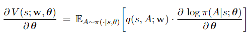
It is not hard to show the policy gradient is
The policy network will be updated using (stochastic) policy gradient ascent. The value network can be updated using temporal different (TD) learning. The following summarizes one iteration of the algorithm.
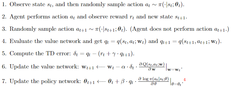
When learning the policy network (actor), the supervision is not from the rewards; instead, the supervision is from the critic's output $q_t=q\left(s_t, a_t ; \mathbf{w}_t\right)$. The actor uses the critic's judgments to improve her performance. When training the critic, the supervision is from the rewards. The critic uses ground truth from the environment to make his judgment more accurate.
# Deterministic Actor-Critic Method
Throughout, the policy function is defined as the probability density function $\pi(a \mid s)$, and the action is randomly sampled according to $\pi$. Deterministic policy is a function that maps state to actions: $\pi: \mathcal{S} \mapsto \mathcal{A}$, where $\mathcal{S}$ is the state space and $\mathcal{A}$ is the action space. Given the state s, the policy function deterministically outputs action $a=\pi(s)$. Deterministic policy is very useful when the actions are continuous.
Deterministic actor-critic method [1] has two networks: policy network $\pi(s ; \theta)$ and value network $q(s, a ; \mathbf{w})$; see Figure 2 . The agent is controlled by the policy network which deterministically maps state $s$ to action $a$. The value network is used for providing the policy network with supervision. The two networks can be trained in the following way.
**The value network can be trained by temporal different (TD) learning.** Let $q_t=$ $q\left(s_t, a_t ; \mathbf{w}_t\right)$ be the prediction and $y_t=r_t+\gamma \cdot q\left(s_{t+1}, a_{t+1} ; \mathbf{w}_t\right)$ be the TD target. The TD crror is $\delta_t=q_t-y_t .$ The model parameters $\mathbf{w}$ can be updated by $\mathbf{w}_{t+1} \longleftarrow \mathbf{w}_t-\left.\alpha \cdot \delta_t \cdot \frac{\partial q\left(s_t, a_t ; \mathbf{w}\right)}{\partial \mathbf{w}}\right|_{\mathbf{w}=\mathbf{w}_t} .$
**Train the policy network by deterministic policy gradient (DPG)** which is totally different from the policy gradient we studied previously. Note that the value network $q\left(s_t, a_t ; \mathbf{w}\right)$ evaluates how good it is for the agent to perform action $a_t$ at state $s_t$. The policy network has motivation to update its parameters $\boldsymbol{\theta}$ so that the action $a_t=\pi\left(s_t ; \boldsymbol{\theta}\right)$ will get a higher evaluation. Intuitively speaking, the policy network (actor) wants to change herself so that the evaluation given by the value network (critic) will increase. The derivative of the objective, i.e., $q\left(s_t, a_t ; \mathbf{w}\right)$, w.r.t. the policy network's parameters $\theta$ is
$$
\mathbf{g}(\theta)=\frac{\partial q\left(s_t, \pi\left(s_t ; \theta\right) ; \mathbf{w}\right)}{\partial \theta}=\left.\frac{\partial \pi\left(s_t ; \theta\right)}{\partial \theta} \cdot \frac{\partial q\left(s_t, a ; \mathbf{w}\right)}{\partial a}\right|_{a=\pi\left(s_t ; \theta\right)},
$$
where the second identity follows from the chain rule. The policy network is updated by performing gradient ascent: $\theta_{t+1} \longleftarrow \theta_t+\beta \cdot \mathbf{g}\left(\theta_t\right)$.
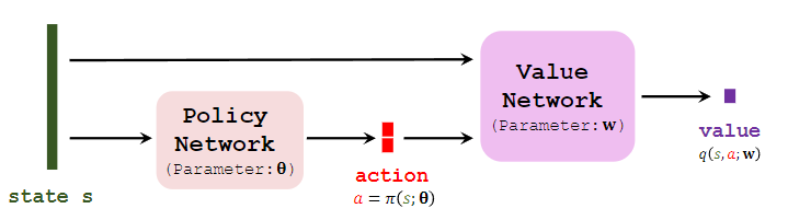
*Figure $2:$ Deterministic actor-critic method. The deterministic policy network maps state $s \in \mathcal{S}$ to action $a \in \mathcal{A} \subset \mathbb{R}^2$. The two dimensions of $a$ are, for example, the stecring angle and accelcration of a self-driving car. The value network maps the pair $(s, a)$ to a scalar.*