📖 Policy-based Deep RL
The policy function $\pi(a \mid s)$ can be used to control the agent: observing the state $S_t=s_t$, the agent randomly samples an action:
$$
a_t \sim \pi\left(\cdot \mid s_t\right) .
$$
The policy function can be approximated by the neural network $\pi(a \mid s ; \theta)$ where ${\theta}$ captures the model parameters. The neural network is called **policy network**.
There are different designs of network architecture. Here, we also consider the game Super Mario, in which the the action space is discrete: $\mathcal{A}=\{$ "left", "right", "up" $\}$. The policy network takes observed state s (which can be a screenshot) as input. The architecture can be
State $\Rightarrow$ Conv $\Rightarrow$ Flatten $\Rightarrow$ Dense $\Rightarrow$ Softmax $\Rightarrow$ Probabilities.
In the Super Mario example, DQN outputs a 3-dimensional vector, e.g., $\mathbf{p}=[0.2,0.1,0.7]$, whose entries corresponds to the three actions. Then the action will be randomly sampled:
$$
\mathbb{P}(A=\text { "left" })=0.2, \quad \mathbb{P}(A=\text { "right" })=0.1, \quad \mathbb{P}(A=\text { "up" })=0.7 .
$$
All of the three actions may be selected. If the random sampling is independently repeated 1000 times, then around 200 observations of $A$ are "left", around 100 are "right", and around 700 are "up".
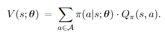
The policy network can be learned using policy gradient algorithms. If the actions are discrete, then the state-value function can be written as 3.1:
$$
V_\pi(s)=\sum_{a \in \mathcal{A}} \pi(a \mid s) \cdot Q_\pi(s, a) .
$$
Policy-based learning uses the policy network $\pi(a \mid s ; \theta)$ to approximate the policy function $\pi(a \mid s)$. With the approximation of policy function, $V_\pi(s)$ is approximated by
Policy gradient is the derivative of $V(s ; \theta)$ w.r.t $\theta$.
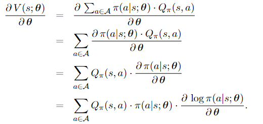
Here, the third identity follows from that $Q_\pi(s, a)$ does not depend on $\theta ;{ }^1$ the last identity follows from that $\frac{\partial \log f(x)}{\partial x}=\frac{1}{f(x)} \cdot \frac{\partial f(x)}{\partial x}$. The above equation can be equivalently written as 3.2:
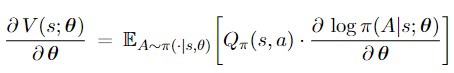
Recall that the approximate state-value function $V(s ; \theta)$ indicates how good the situation $s$ is if policy $\pi(a \mid s ; \theta)$ is used. We thereby have the motivation to update $\theta$ so that $V(s ; \theta)$ will increase (which means the situation is better.) Thus, the policy network can be updated by policy gradient ascent:
$$
\theta_{t+1} \longleftarrow \theta_t+\left.\beta \cdot \frac{\partial V(s ; \theta)}{\partial \theta}\right|_{\theta=\theta_t},
$$
where $\beta$ is the learning rate.
To this end, we defined the policy network and derived the policy gradient in (3.2). However, there are two unsolved problems. First, the expectation in (3.2) maybe intractable; this is typically
the case when the action space $\mathcal{A}$ is continuous, e.g., $\mathcal{A}=[0,1]$. Second, the action-value $Q_\pi(s, a)$ is unknown. We answer the two questions one by one.
**What if the expectation in (3.2) is intractable?** If the action space $\mathcal{A}$ is continuous, then the expectation (which is an integration) is typically intractable. Given state $S_t=s_t$, if the action $A_t=a_t$ is randomly sampled according to the $\text{PDF} \space \pi\left(\cdot \mid s_t ; \theta\right)$, then
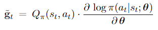
is an unbiased estimate of $\frac{\partial V\left(s_t ; \theta\right)}{\partial \theta}$. We can think of $\mathrm{g}_\theta(\theta)$ as a stochastic gradient and update $\theta$ using stochastic gradient ascent.
How do we know the action-value $Q_\pi(s, a)$ ? There can be two solutions: first, use the observed return $r_t$ instead of $Q_\pi(s, a)$; second, approximate $Q_\pi(s, a)$ using a neural network. The two solutions are described in the following:
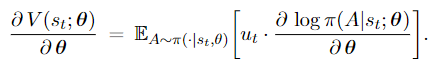
- Play a game to the end, obtain all the rewards $r_1, r_2, \cdots, r_T$, and compute the returns $u_1, u_2, \cdots, u_T$ using the equation $u_t=\sum_{i=t}^T \gamma^{i-t} \cdot r_i$. Since $Q_\pi\left(s_t, a_t\right)=\mathbb{E}\left[U_t \mid s_t, a_t, \pi\right]$, we can use $u_t$ to replace $Q_\pi\left(s_t, a_t\right)$. In this way, the policy gradient (3.2) at time step $t$ becomes
AlphaGo [2] uses this approach.
- Use a value network to approximate $Q_\pi(s, a)$. The value network provides supervision to the policy network. The value network can be learned by temporal difference (TD). This leads to the actor-critic method which is elaborated on in Section 4.1.
**Remark**: *The derivation of policy gradient written in the above is not rigorous! It is a simplified version to make the policy gradient easy to understand. To be rigorous, we must take into account that $Q_\pi$ depends on the policy $\pi$ and is thereby a function of $\theta$. However, even is $Q_\pi$ 's dependence on $\theta$ is taken into account, the resulting policy gradient is the same to (3.2).*