🔖 Notation
Throughout, we use uppercase letters, e.g., $X$, to denote random variables and lowercase letters, e.g., $x$, to denote their observations. Let $\mathbb{P}(X=x)$ be the probability of the event " $X=x$ ". Let $\mathbb{P}(Y=y \mid X=x)$ be the probability of the event " $Y=y$ " under the condition "X $=x$ ".
**Agent**: A system that is embedded in an environment and takes actions to change the state of the environment. Examples include robots, industrial controllers, and Mario in the game Super Mario.
**State $(S)$** : State can be viewed as a summary of the history of the system that determines its future evolution. State space $\mathcal{S}$ is the set that contains all the possible states. At time step $t$, the past states are observed and we thus know their values: $s_1, \cdots, s_t$; however, the future states $S_{t+1}, S_{t+2}, \cdots$ are unobserved random variables.
**Action $(A)$** : The agent's decision based on the state and other considerations. Action space $\mathcal{A}$ is the set that contains all the actions. Action space can be a discrete set such as \{ "left", "right", "up" $\}$ or a continuous set such as $[0,1] \times[-90,90]$. At time step $t$, the past actions are observed: $a_1, \cdots, a_t$, but the future actions $A_{t+1}, A_{t+2}, \cdots$ are unobserved random variables.
**Reward $(R)$** : Reward is a value received by the agent from the environment as a direct response to the agent's actions. At time step $t$, all the past rewards are observed: $r_1, r_2, \cdots, r_t$. However, the future reward $R_i$ (for $i>t$ ) is unobserved, and it depends on the random variables, $S_{t+1}$ and $A_{t+1}$. Thus, at time step $t$, the future rewards $R_{t+1}, R_{t+2}, \cdots$ are random variables.
**Policy function $(\pi)$** : The decision-making function of the agent. Policy is the probability density function (PDF): $\pi(a \mid s)=\mathbb{P}(A=a \mid S=s)$. The policy function maps the observed state $S=s$ to a probability distribution over all the actions in set $\mathcal{A}$. Since $\pi$ is a PDF, $\sum_{a \in \mathcal{A}} \pi(a \mid s)=1$. The agent will perform action $a$ with probability $\pi(a \mid s)$, for all $a \in \mathcal{A}$. See the illustration in Figure 1 .
**State transition $(p)$** : Given the current state $S=s$, the agent's action $A=a$ will lead to the new state $S^{\prime}$ given by the environment. State-transition function is the probability density function (PDF) $p\left(s^{\prime} \mid s, a\right)=\mathbb{P}\left(S^{\prime}=s^{\prime} \mid S=s, A=a\right)$. The environment makes $s^{\prime}$ the new state with probability $p\left(s^{\prime} \mid s, a\right)$, for all $s^{\prime} \in \mathcal{S}$.
**Trajectory**: The agent's interaction with the environment results in a sequence of (state, action, reward) triplets: $s_1, a_1, r_1, s_2, a_2, r_2, s_3, a_3, r_3, \cdots$
**Return $(U)$** : Return (aka cumulative future reward) is defined as
$$
U_t=R_t+R_{t+1}+R_{t+2}+R_{t+3}+\cdots
$$
**Discounted return** (aka cumulative discounted future reward) is defined as
$$
U_t=R_t+\gamma \cdot R_{t+1}+\gamma^2 \cdot R_{t+2}+\gamma^3 \cdot R_{t+3}+\cdots
$$
Here, $\gamma \in(0,1)$ is the discount rate. The return $U_t$ is random because the future rewards $R_t, R_{t+1}, R_{t+2}, \cdots$ are unobserved random variables. Recall that the randomness in the $R_i(i \geq t)$ comes from the future states $S_i$ and action $A_i$.
**Action-value function** $\left(Q_\pi\right)$ : Action-value function $Q_\pi\left(s_t, a_t\right)$ measures given state $s_t$ and policy $\pi$, how good the action $a_t$ is. Formally speaking,
$$
Q_\pi\left(s_t, a_t\right)=\mathbb{E}\left[U_t \mid S_t=s_t, A_t=a_t\right] .
$$
The expectation is taken w.r.t. the future actions $A_{t+1}, A_{t+2}, \cdots$ and future states $S_{t+1}, S_{t+2}, \cdots$ which are random variables. Note that $Q_\pi\left(s_t, a_t\right)$ depends on the policy function $\pi$ and the statetransition function $p$.
**Optimal action-value function** $\left(Q^{\star}\right)$ : The optimal action-value function $Q^{\star}\left(s_t, a_t\right)$ measures how good the action $a_t$ is at state $s_t$. Formally speaking,
$$
Q^{\star}(s, a)=\max _\pi Q_\pi(s, a) .
$$
Note that $Q^{\star}(s, a)$ is independent of the the policy function $\pi$.
**State-value function $\left(V_\pi\right)$** : State-value function $V_\pi\left(s_t\right)$ measures given $\pi$, how good the current situation $s_t$ is. Formally speaking,
$$
V_\pi\left(s_t\right)=\mathbb{E}_{A \sim \pi\left(\cdot \mid s_t\right)}\left[Q_\pi\left(s_t, A\right)\right]=\int_{\mathcal{A}} \pi\left(a \mid s_t\right) \cdot Q_\pi\left(s_t, a\right) d a .
$$
Here, the action $A$ is treated as a random variable and integrated out.
**Optimal state-value function $\left(V^{\star}\right)$** : The optimal state-value function $V^{\star}\left(s_t\right)$ measures how good the current situation $s_t$ is. Formally speaking,
$$
V^{\star}(s)=\max _\pi V_\pi(s) .
$$
Note that $V^{\star}(s)$ is independent of the the policy function $\pi$.
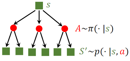
*Figure 1: Illustration of the randomness. The action $A$ is randomly sampled according to the policy function. The new state $S^{\prime}$ is randomly sampled according to the state-transition function.*